CVD 3a -Rolling Accel (simple)
To many, the ability to accelerate in a big and exciting fashion, is what puts the Race in Race Car.
In this chapter we’ll examine what makes cars accelerate, how we can quantify the acceleration value, and how to compare those values between cars. In doing so hopefully we can dispel some of the myths and misconceptions out there, and provide the reader a more comprehensive way of looking at acceleration. How many times have we read an article or message board thread entitled “HP vs. torque”, or heard “Horsepower sells cars, torque wins races” ? Many people out there are convinced that the car with more torque, must accelerate better at lower speeds, or the higher hp car will be faster at higher speeds?
The truth is, the nature of a car’s acceleration can’t really be cast right into one of these buckets. Every car, in every state of tune, possesses a unique character of acceleration, driven by many factors. An effective comparison must take many factors into account to paint a complete and accurate picture. To start, for each car, you must collect several ingredients-
PART ONE: COLLECT THE RAW DATA
Race weight of the car
This should probably include a static driver weight in each car to produce a more realistic result.
Diameter of the driving tires
You can calculate what it *should* be – for instance, a 225/45-17 should be ((17 inches ) + ((225mm)*.45)*2)) = (17″ + (101.25mm)*2) = (17″ + 202.5mm) = 17″ + 7.97″ ~=25″ in diameter. Usually a tire manufacturer will provide a diameter value to save you that trouble, but even better if available, is a “Revs per mile” value. This is based more on the effective loaded radius of the tire, and provides what I’ve found to be the best approximation of actual diameter – it will also plug more easily into our formulas later.
Final drive ratio
For rear drive cars, this is the gear in the rear end, FWD cars have it in their transmission cases.
Gear ratio
Of the gear we’ll be in for the comparison. If multiple gears are to be used, we’ll have to look at each one of them individually.
Output of the engine
What we need here is a dyno showing the torque curve of the engine, covering the engine RPM range within which it’ll be operating. If we’re looking to do a comparison of 600cc superbikes or F1 engines, we might not care about anything below 7000rpm. If we’re looking at diesel truck engines, we probably won’t be looking over 4000rpm. For most production car engines, we’re looking to see what they produce from around 2500rpm to their redline. If you only have a hp curve, you can reverse-engineer the torque values through the formula:
HP = (TQ *RPM)/5252Now, this isn’t to say torque is more important than horsepower, or that one is only a “derived value” or that “the dyno measures (torque or horsepower), therefore (horsepower or torque) is a meaningless measure”, etc. etc. If you’ve ever seen one of these hp vs. tq threads, you’ve seen all these sorts of statements. The reality is, we don’t care about any of that – we just need a torque curve to go to the next step.
One thing that’s very important, is that we need to know a little bit about the device that produced the measurement, and we have to do our best to build in some correction for this. There are many different types of chassis dyno – the Dynojet, the Mustang Dyno, and the Dynapack being the three most popular. The former two have the car’s tires spinning up rollers, while the latter attaches directly to the vehicle’s hubs. In my experience, the Dynapack generally produces slightly higher readings, but it’s well within the calibration/error range of different dynos – the operator has the ability to implement correction and calibration adjustments to make the numbers higher or lower as they see fit. Every dyno has to be observed with a grain of salt; the more you know about the dyno, what sort of results it’s produced before for known-quantity cars, and the conditions of the dyno test, the better a comparison you’ll be able to make. The other type of dyno is an engine dyno, where the engine is tested out of the car – for this you have to take into account a driveline loss factor, if you wish to compare to cars measured on a chassis dyno. This can be anywhere from 10-20%, and it depends a lot on the drive type (AWD will generally have higher losses than FWD or RWD) and power levels – as power levels go up, driveline loss percentages go down. A transmission and rearend pair sapping 50hp from a 500hp engine, probably won’t sap an extra 50hp when a 1000hp engine is put in front of it.
Speed range in question
This is something often overlooked yet super critical. Since we’re looking at rolling acceleration, we’re going to ignore the first 10-15mph, since that falls into the launch category which we’ll cover later. The big hurdle many can’t get over, is the car with better power:weight ratio, won’t necessarily out-accelerate a car with an inferior power:weight ratio, at all speeds. Power:weight ratios are calculated based on peak power – when we do our comparison, it’ll be between two cars through a speed range, and while the car with better power:weight probably out-accelerates the inferior ratio’d car somewhere, it doesn’t necessarily occur in the speed range we care about.
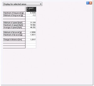
Speed range – autocrossIn last chapter we broke down an autocross run into its essential elements, or “events”, and showed their proportional weight to the overall time. Using the same data collected earlier, we can produce some simple summarized statistics about the run:
Again, the run we chose was a superb example of a typical Nationals course. On it, the SS Viper had a minimum speed of 31mph, a maximum speed of 70mph, and an average speed of 48.2mph. Over the course of the run we covered 1.25km, or a bit under 8/10ths of a mile. Dividing the distance traveled by average speed gets us back to our timeslip’s data point of 58.0 seconds elapsed.
Using this knowledge, we can figure out the average speed of any of the other classes, since they ran the same course. Choosing one at random, say STX. The quick clean STX time on that same course was 61.692 seconds. (.775 miles/61.692 seconds)*(3600 seconds/hour) which works out to a 45.2mph average speed – only 3mph slower. That’s right – a 115hp Honda Civic on street tires, is only 3mph slower around a Nationals autocross course, than a 505hp Viper on race tires. Of course, if you look up the speed ladder to Jeff Kiesel’s tiny E-Modified Sprite, the fastest production-based car at Nationals this year, it ran a 54.6 time on that same course, working out to 51.1mph, just under 3mph faster than the Viper.
So 30-70mph is the range seen by an SS Viper. A car with a 3mph slower average won’t necessarily care about 27-67mph, would depend on the nature of the car. Some cars (like the Viper) have relative big power and tall enough gearing to hit high speeds when given the opportunity; others make their time by being quicker in the handling sections. The point is, even across as wide a range as STX to EM, we’re looking at less than a 6mph average speed difference. High 20’s -> mid 60’s is the speed range we care about in autocross. With an average speed in the mid to upper 40’s, the most important part of our car’s acceleration “character”, is how it behaves around that average speed. Acceleration below 25mph, or above 70mph, while nice, really isn’t important.
Speed range – trackThe speed range we care about at the track is much much wider, and every track we enter will have a different speed range. Unlike autocross, we know we’re going to be shifting while on the track, so we need to be looking at our acceleration in different gears. We need to maintain good pull out of the slowest corner on the track, but not run out of gears and hit an artificial top speed too early in the fast section.
Optimization and comparisons of acceleration as applied to the track is much more complicated than autocross. Each must be done on a track-by-track basis. The good news is you can collect data for a given track, and based on that, you’ll have a good idea of corner exit speeds from each corner, so your acceleration optimization can use those starting speeds as a reference. Paul Van Valkenburgh did a great job explaining the optimization of gearing for the track in his Race Car Engineering & Mechanics so I won’t be going through that here.
PART TWO: PLUG IN THE DATA
Most reading have a pretty good idea of what happens to make your car go but we’ll go through it briefly again here to explain why we needed each piece of data, each bolded.
Air and fuel inside your engine ignites and produces an extremely intense explosion. This explosion is contained by the engine cylinder block and head, which forces the piston to move downward. The force from this explosion pushing on the piston, turns the crankshaft in the engine. Our engine’s torque/horsepower output tells us how much force we’re able to produce at the end of our crankshaft. From there, the forces go through the flywheel, clutch, and pressure plate, to the transmission’s input shaft. Inside the transmission, our force is either multiplied by some amount (trans gear ratio >1), passed straight through (1:1), or reduced, as in an overdrive (ratio <1). Out the transmission to the final drive, where again our force is multiplied by our final drive ratio – usually something in the 2.xx to 4.xx range.
So by the time the output of our exploded air and fuel reaches our drive axles, its effect has been multiplied by our transmission ratio, and again by our final drive ratio. If you had a 2:1 gear in the transmission and a 4:1 final drive ratio, then a 10 ft-lb. input twist to the transmission, would produce 80ft-lbs. of torque at the drive axles. The problem is, for every degree of rotation of our drive axles, we have to rotate our input shaft 8 degrees – a full turn of our input shaft only produces 1/8th of a turn. If we had a “taller” final drive, or shifted to a higher gear, then we might get more than 1/8th of a turn, but our torque multiplication would be reduced. This is why our cars produce more acceleration in the lower gears – it’s not just aero drag.
So at this point we know the force available at our drive axles, but they still have a way to go to start moving the car. Out at the end of the axles are our wheels and tires. Just like a gear reduction, the taller, or larger diameter, our wheels and tires, the more the forces from our engine will be reduced. We need to know the diameter of our driven tires to know how much of a reduction occurs.
All of these explosions and twisting and gears and shafts aren’t going to do us any good if we’re not on the ground, the car will sit there. We’re dependent upon that magical interaction between the tire and the ground, at our little contact patches. Newton’s third law states that for every force, there is an equal and opposite force. Well, in order for our car to push our car in one direction, we’re going to have to push the earth back the other way!
Fortunately the earth weighs a bit more than our car, so it continues at the same speed, and our car accelerates. But how much does it accelerate? Going back to Newton with his Second Law, we know that Force = Mass * Acceleration. As we went through above, our engine’s torque output at the crank is multiplied by the transmission, multiplied again by the rear end, then multiplied (or divided) by the height of our driving tire – all that business gives us the Force we have available. We also know the Mass of our car, so we have everything we need to solve for our Acceleration. Now let’s walk through an example of a single data point.
So let’s say we’re driving in second gear, and the engine is at 4500rpm, where it makes 335ft-lbs. of torque at the drive axles. If the second gear ratio is 2.07, the final drive ratio is 3.42, then the actual torque at the drive axles is 335 x 2.07 x 3.42 = 2371 ft-lbs. If our tire was 24″ in diameter, then the radius of the tire is 12″ (or 1 foot), so the force pushing on the earth is 2371ft-lbs / 1ft = 2371lbs. If our car weighed 2371 pounds, then we would get a theoretical** 1g acceleration!
**There are a few variables that will combine to make our actual measured/experienced real-world acceleration different (usually lower) than what we predict using the simplest version of this method. They’ll be discussed more later.
Continuing our 2371ft-lb. example above (all these numbers are stock C5 Z06 values), we’ll use instead a drive tire of 315/30-18, with a diameter of about 25.6″. So instead of having 2371pounds of force (aka thrust), we’re going to have 2371 * (12/(25.6/2)) = 2371 * (12/12.8) = 2371 * (.9375) = 2222 pounds of force. The lesson here, is a tire is a “gear” in the works, just like our transmission gear and final drive – making the tire taller reduce the forces we’ll produce with all else equal, but in turn, the taller tire will allow a higher speed at the same RPM.
So our stock C5 Z06 @3050lbs, at 4500RPM full throttle, experiences a theoretical (2222lbs/3050lbs) = .728g of thrust. That little “g” in there is a unit of acceleration, equal to the acceleration an object experiences due to gravity. If you drop an object at sea level, in a vacuum (no aero drag), it will accelerate towards the ground at 1g. Wikipedia has a good explanation of g-force if you’d like further reading.
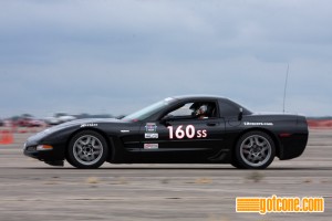 (Jason Munchhof’s Z06 accelerating at the 2010 SCCA Solo Nationals)
Now to speed – we know we’re at 4500RPM, and producing a theoretical .728g of longitudinal (forward) acceleration. But where are we in the speed range we care about? Could be we’re already going too fast, or still too slow.
To know our speed at a given RPM in a given gear, we have to convert a bunch of units. If we know the revs/mile of our tire that saves some work. Our 315/30-18 *should* have a revs/mile of around 788. If the value isn’t published, we *should* be able to figure how many revs happen in one mile for our tire based on its stated size or diameter. In one rev it *should* cover a linear distance equal to its circumference – pi (3.1415927) times the diameter (pi * 25.6) = 80.424″, or 6.7 feet. We know a mile is 5280 feet, so we should require (5280/607) ~788 revs per mile. There’s a lot of *should*s in there because in reality, we might cover a few more or a few less, depending on how the tire is constructed, the speeds we’re going, even the air pressure we use.
So, our engine is turning 4500RPM, we’re in second gear (2.07 ratio), have a final drive ratio of 3.42, and our tire needs 788 revolutions to cover one mile. What is our speed?
In units, we have revolutions per minute from the engine, and revolution/mile from the tire. In the end, we want to get to miles per hour for the car as a whole.
First thing we have to do is “flip” the revolutions/mile so instead of 788revs/mile, we have 1/788 miles per revolution. Revs/minute * miles/rev cancels out revs, and gives us miles/minute. Since we usually talk about MPH, Miles Per Hour, we need to multiply our engine RPM by 60 to give us RPH, revolutions per hour, so our final units work out to miles/hour. Here we go-
(4500revolutions/minute)*60 minutes/hour = 270,000 revolutions/hour
our gear reduction is 2.07 * 3.42 = 7.0794, so unlike the eninge, our drive axles only turn at (270,000/7.0794) = 38,138 revolutions/hour
we know our tires move us 1/788th of a mile per revolution, so our ground speed, at 4500mph in second gear, is-
38,138 revolutions/hour * 1/788 miles/revolution = 38,138/788 miles/hour = 48.4MPH. Whoo! Now we know the C5 Z06 is capable of .728g of acceleration not just at 4500RPM, but also at 48MPH, which happens to be a very important speed on the autocross course, darn near exactly our average speed.
There was a lot of work put into producing this single data point. Most of this was done to explain the process, which works for any car, at any RPM, and fortunately we have some tools at our disposal to help in the automation of this analysis, and to provide graphs, showing how the acceleration of a given car compares to others. Microsoft Excel is one such tool.
Jason’s CVD acceleration worksheet available for download here: CVD_thrust
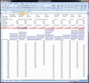
Here’s a screenshot of the Data tab, where you plug in the car data:
All of these values have been covered above. There’s a “dyno adjust” variable built in, that you can use to fine-tune things up or down, if you think a dyno or its operator might have been off in its process. There’s a place to include a link to the source dyno for reference. The bottom portion is where we take the torque curve for the car in question, and put it into the spreadsheet. I use data points every 250RPM along the way, this tends to produce a relatively smooth curve, where there’s not likely to be any huge dips or bumps between our data points.
PART THREE: ANALYZE THE OUTPUT
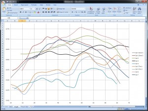
The curves themselves are present on the second “Graph” tab:
This is really the fruit of all this labor, the place to spend the most time looking at things. These wacky lines are showing us the true nature or “character” of acceleration that we sought to find from the beginning. Big or small, heavy or light, torque or horsepower – this is the graph that will tell you which car is faster, and where. The horizontal, or “X” axis, shows our speed in MPH. The vertical “Y” axis shows how hard our car is accelerating. There is no more magic beyond this – it doesn’t matter if one car has 12 cylinders and the other 4; if one car makes 500hp (or ft-lbs. of torque!) and the other only 200; one car weighs 4000 pounds and the other only 2000; whichever car has the higher line is going to accelerate harder than the other car, and pull ahead, no matter what any other factor may suggest.
There’s a few ways we can use this analysis to help guide our decisions in tuning. For autocross, does our line, in second gear, end at a too-low speed? If so, we’ll either need to use third gear, or maybe want to consider raising the limiter, raising our gearing, or getting a taller drive tire. If our line ends at much-too high a speed (80+mph) and the thrust values are lower than we’d like, then shorter gearing, or a shorter drive tire, may be of benefit. We can plug in different gear ratios or tire diameters, or fiddle with dyno numbers to represent a planned engine mod, and instantly see in the graph, how this will affect our acceleration versus our competitors.
For the track, you’ll want to plot multiple lines for each car, one for each gear the car will use while on the track. The speed at which a gear’s line crosses under the next higher gear, is a good shift point. If it never reaches the next line, then it makes sense to wind it to redline. We can do some other tricky stuff too – if we’re going to control the speed of a rolling-start wheel-to-wheel race, we want to choose a speed where we’ve got better acceleration than our competitor, or perhaps a speed where they’ll be forced to shift soon after the start. Of course, knowing this requires us to do the complete data collection steps for each of our competitor’s cars.
The sample data provided in the spreadsheet shows several different acceleration profiles for SCCA Solo Super Stock cars. The Viper, C5 Z06, C6 Grand Sport, 911 GT3, Lotus Elise, and a potential future SS competitor, the Audi R8. You might be able to pick out the Lotus in looking at the graph, but might be surprised to find how some of the others actually end up.
As covered in Chapter 2, longitudinal acceleration only comprises about 10% of our time on an autocross course so it’s far from the most important factor. However, when everything else is very close, it can be a deciding factor when most championships are won by a few tenths. This step of analysis demonstrates which car holds the advantage in the “rolling acceleration” event in our Septathlon of autocross.
PART FOUR: SOME OTHER VARIABLES TO CRASH THE PARTY
As mentioned above with the “**”, there’s a few other things that come into play but are smaller in their contribution to the outcome, and may be harder or less fun to find. Even though our rolling acceleration is by far the simplest thing to analyze and quantify that our car does, it is still rather complex, as evidenced by the already long length of this chapter. These party-crashing variables include:
- Aerodynamic drag of the car. You can calculate this using the car’s coefficent of drag (cD) and its frontal area. This isn’t too big a factor at autocross speeds but would come into play at a big track or to a freeway racer (shame on you!). If you were an enterprising individual, you could find these drag numbers, and add them to the existing acceleration worksheet, and have them automatically reduce the acceleration as a function of speed. Since the focus is mainly on autocross speeds where the drag contribution is rather minimal, I have not done so here.
- Mechanical drag. Even when we’re coasting, our brakes might be dragging a little, our tires are being heated up a bit and dragging on the pavement, especially if we have a lot of toe (in or out) in our alignment. The only really good way to figure this out is to do some careful coast-down tests. Find a flat stretch of road, and using your data acquisition system, measure how long it takes for the car to decelerate from one low speed to another – like 40mph to 20mph. Do this test several times to get an accurate value. This will give you an idea of an always-present mechanical drag value that will decrease your achieved acceleration. As with aero drag, this too, could be built into the spreadsheet. The value would be attainable for your car but hard to get for others.
- When we accelerate the car, we’re accelerating the mass of the car, but we’re also spinning up our front wheels/tires and brake rotors, which we didn’t do on the dyno. This takes more energy from the system, and again affects our achieved real-world acceleration vs. what our calculations tell us is possible. If our chassis dyno was of an AWD car spinning up two sets of rollers, then maybe this won’t factor in.
- Difference between output as measured on the dyno, vs. what’s achieved in the real world. Cars are dyno’d while sitting still in a shop, usually with the hood up and a fan going. This is a much different environment than rolling along on the road with the hood closed. In most cases the car will probably make a little more power on the dyno than on the road, but there are some vehicles that use ram-air type systems that theoretically could boost the performance at speed.
While these variables all certainly matter, they tend to cancel each other out across cars, for the most part. While one could go to great lengths to find these values and plot them, at autocross speeds anyway, it’s probably just best to figure that any two acceleration curves within a few percent of each other, are more or less equal, based on the contribution of these variables. An analysis at a high-speed track would certainly benefit from the aerodynamic drag component however.
PART FIVE: OH NO, NOT ANOTHER VARIABLE??
There is one other lurking variable to consider that we haven’t touched on yet. I had really hoped to not have to talk about grip until the skidpad chapter, as explaining tires is difficult and complicated. However, this acceleration analysis isn’t complete without acknowledging the fact that a car won’t always be able to achieve its theoretical acceleration – if it spins the tires first! A car’s longitudinal grip limit places a “ceiling” on how high its real-world longitudinal acceleration can go. A car that runs into this problem is described as “traction limited”, where the available grip determines the maximum possible acceleration, while in most cases, cars are “power limited”, the engine’s output being the limiting factor.
Because of the complexity in explaining grip, I have decided to split the Rolling Acceleration chapters into 3a (simple), and coming next, 3b (complex), where we will introduce grip, tire loading, and weight transfer. There are no precise rules on where grip comes into play, but above about .5g for a FWD car, .8g for a RWD car, grip is something you’ll need to start worrying about. Of course, even those guidelines are dependent upon a whole ‘nother long list of variables we’ll go over in 3b. Stay tuned!
[…] […]